9 Webからのデータ取得（2）「World Bank API」

e-Statは日本の統計データを見る場合に利用しましたが、世界の国別の統計や指標を見たり比較したりする場合には世界銀行のウェブサイトが便利です。世界銀行のデータをAPI経由で取得するためのRのパッケージがwbstatsです。

使っているPCで初めて利用する場合は、

install.packages("remotes")
remotes::install_github("nset-ornl/wbstats")

でインストールしてください。セッションを立ち上げた後（プロジェクトを立ち上げた後）には、

library(wbstats)

を実行してwbstatsの関数が利用できるようにしておきます。wb_cachelistは、利用可能な指標や国、トピックなどの一覧を保持しています。

str(wb_cachelist, max.level = 1)

## List of 8
##  $ countries    : tibble [304 x 18] (S3: tbl_df/tbl/data.frame)
##  $ indicators   : tibble [16,649 x 8] (S3: tbl_df/tbl/data.frame)
##  $ sources      : tibble [63 x 9] (S3: tbl_df/tbl/data.frame)
##  $ topics       : tibble [21 x 3] (S3: tbl_df/tbl/data.frame)
##  $ regions      : tibble [48 x 4] (S3: tbl_df/tbl/data.frame)
##  $ income_levels: tibble [7 x 3] (S3: tbl_df/tbl/data.frame)
##  $ lending_types: tibble [4 x 3] (S3: tbl_df/tbl/data.frame)
##  $ languages    : tibble [23 x 3] (S3: tbl_df/tbl/data.frame)

利用可能な指標の一覧は以下のコマンドで確認できます。

View(wb_cachelist$indicators)

indicator_id	indicator	unit	indicator_desc	source_org	topics	source_id	source
1.0.HCount.1.90usd	Poverty Headcount ($1.90 a day)	NA	The poverty headcount index measures the proportion of the population with daily per capita income (in 2011 PPP) below the poverty line.	LAC Equity Lab tabulations of SEDLAC (CEDLAS and the World Bank).	11 , Poverty	37	LAC Equity Lab
1.0.HCount.2.5usd	Poverty Headcount ($2.50 a day)	NA	The poverty headcount index measures the proportion of the population with daily per capita income (in 2005 PPP) below the poverty line.	LAC Equity Lab tabulations of SEDLAC (CEDLAS and the World Bank).	11 , Poverty	37	LAC Equity Lab
1.0.HCount.Mid10to50	Middle Class ($10-50 a day) Headcount	NA	The poverty headcount index measures the proportion of the population with daily per capita income (in 2005 PPP) below the poverty line.	LAC Equity Lab tabulations of SEDLAC (CEDLAS and the World Bank).	11 , Poverty	37	LAC Equity Lab
1.0.HCount.Ofcl	Official Moderate Poverty Rate-National	NA	The poverty headcount index measures the proportion of the population with daily per capita income below the official poverty line developed by each country.	LAC Equity Lab tabulations of data from National Statistical Offices.	11 , Poverty	37	LAC Equity Lab
1.0.HCount.Poor4uds	Poverty Headcount ($4 a day)	NA	The poverty headcount index measures the proportion of the population with daily per capita income (in 2005 PPP) below the poverty line.	LAC Equity Lab tabulations of SEDLAC (CEDLAS and the World Bank).	11 , Poverty	37	LAC Equity Lab
1.0.HCount.Vul4to10	Vulnerable ($4-10 a day) Headcount	NA	The poverty headcount index measures the proportion of the population with daily per capita income (in 2005 PPP) below the poverty line.	LAC Equity Lab tabulations of SEDLAC (CEDLAS and the World Bank).	11 , Poverty	37	LAC Equity Lab

データの検索はwb_search()関数を用います。

wb_search("forest area")

## # A tibble: 4 x 3
##   indicator_id   indicator                          indicator_desc              
##   <chr>          <chr>                              <chr>                       
## 1 AG.LND.FRST.HA Forest area (hectares)             Forest area is land under n~
## 2 AG.LND.FRST.K2 Forest area (sq. km)               Forest area is land under n~
## 3 AG.LND.FRST.ZS Forest area (% of land area)       Forest area is land under n~
## 4 ER.FST.DFST.ZG Annual deforestation (% of change) Average annual deforestatio~

実際のデータの取得は、wb_data()関数を用います。indicator引数に取得したいデータのIDを指定します。

fa_data <- wb_data(indicator = "AG.LND.FRST.ZS", country = "all")

いくつかの国について、国土面積に対する森林面積の割合の推移を折れ線グラフとしてプロットしてみます。

fa_data %>% 
    filter(country %in% c("Japan", "World", "China",
                                                "Latin America & Caribbean")) %>% 
    mutate(date = lubridate::ymd(date, truncated = 2)) %>% 
    rename(value = 5) %>% 
    filter(!is.na(value)) %>% 
    ggplot(aes(date, value, group = country, color = country)) +
    geom_line() +
    theme_minimal(base_size = 16) +
    theme(legend.position = "bottom") +
    labs(x = "年", y = "森林面積の割合[%]",
             title = "国土面積に対する森林面積の割合の推移") +
    gghighlight(label_params = list(direction = "y"))

## label_key: country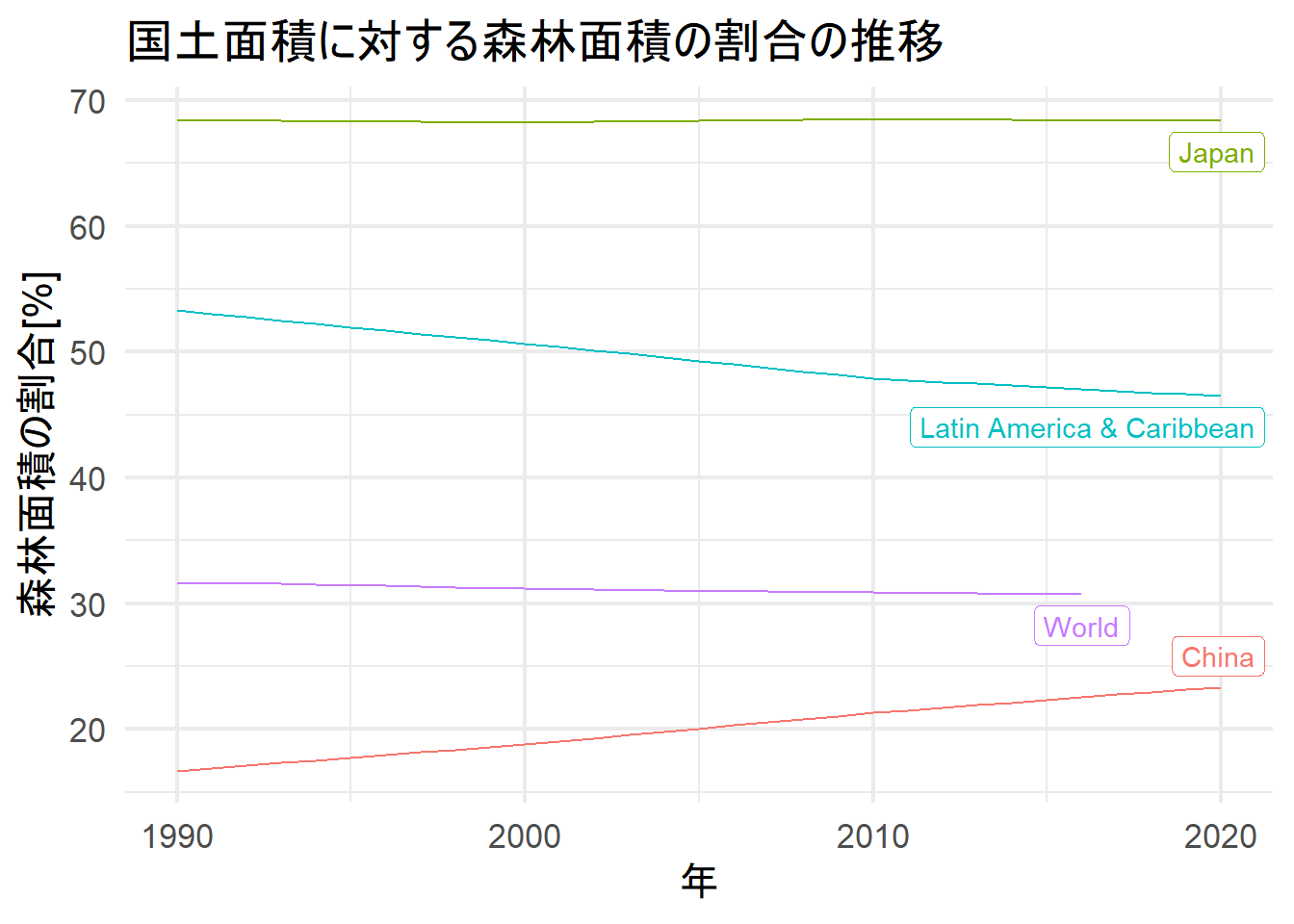

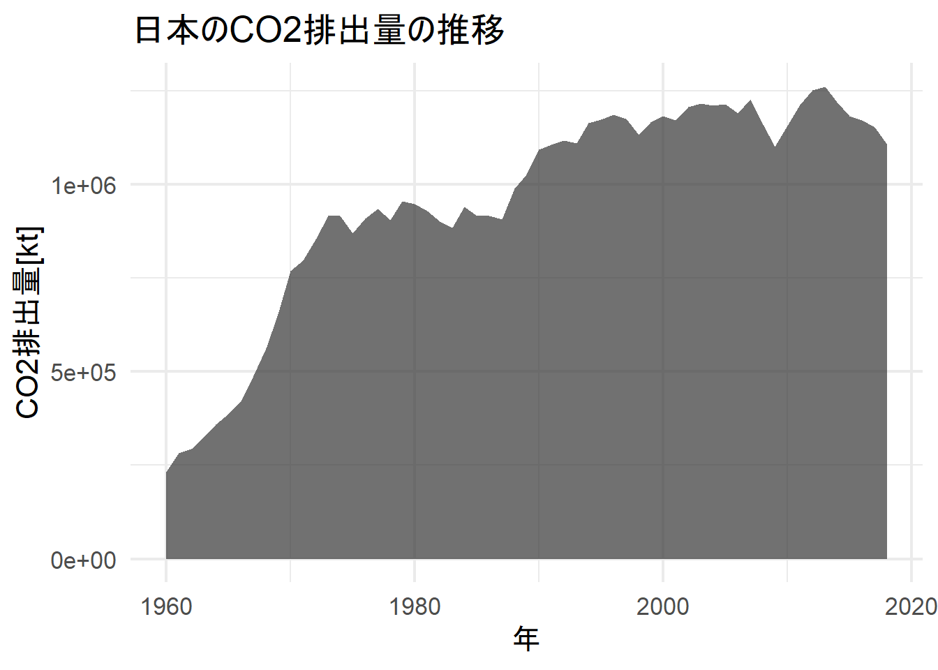
次に、日本のCO2排出量の推移を見てみましょう。

View(wb_search("CO2 emissions"))

co2_data <- wb_data(indicator = "EN.ATM.CO2E.KT")
head(co2_data)

## # A tibble: 6 x 9
##   iso2c iso3c country  date EN.ATM.CO2E.KT unit  obs_status footnote
##   <chr> <chr> <chr>   <dbl>          <dbl> <chr> <chr>      <chr>   
## 1 AW    ABW   Aruba    1960         11093. <NA>  <NA>       <NA>    
## 2 AW    ABW   Aruba    1961         11577. <NA>  <NA>       <NA>    
## 3 AW    ABW   Aruba    1962         12713. <NA>  <NA>       <NA>    
## 4 AW    ABW   Aruba    1963         12178. <NA>  <NA>       <NA>    
## 5 AW    ABW   Aruba    1964         11841. <NA>  <NA>       <NA>    
## 6 AW    ABW   Aruba    1965         10623. <NA>  <NA>       <NA>    
## # ... with 1 more variable: last_updated <date>

co2_data %>% 
    filter(country == "Japan") %>% 
    mutate(date = lubridate::ymd(date, truncated = 2)) %>% 
    rename(value = 5) %>% 
    filter(!is.na(value)) %>% 
    ggplot(aes(date, value)) +
    geom_area(alpha = 0.7) +
    theme_minimal(base_size = 16) +
    labs(x = "年", y = "CO2排出量[kt]",
             title = "日本のCO2排出量の推移")